Interpolative Algorithms vs. Truncated Inverse FFT: A Comparative Study

Table of Links

Abstract & Introduction

Optimization of the Optical Interpolation

Materials and Methods

Results and Discussion

Conclusion

Appendix A: Proof of Hermitian Self-Adjoint product identity for Equidistant Time-Domain Measurements

Appendix B: AAH ̸= MIN I in the Non-Equidistant Case

Acknowledgments & References

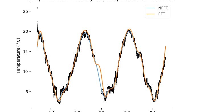
4 RESULTS AND DISCUSSION

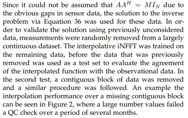
All training data were mean-centred prior to analysis; and the means were added to the reconstructed data prior to recording the residuals. The results summarise cross validation routines for randomly sampled data in Table 4, and randomly sampled contiguous blocks in Table 4 at 3 levels of missing data (10, 20, and 30%) performed for a total of 7 times to get the average error, and the uncertainty, as one standard deviation associated with the error measurement. Both relative error for the predicted set, and the correlation coefficient for the reconstructed data on the full data set, versus the partially sampled dataset were also performed to intuit the error due to the constraint of the reconstruction (via the weighted kernel approximation) versus the sparsity of the observed data.

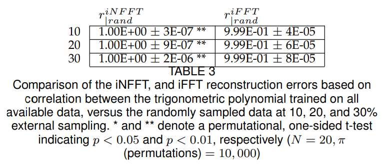
The relative error for the randomly sampled data is on the same order of magnitude as reported in the original

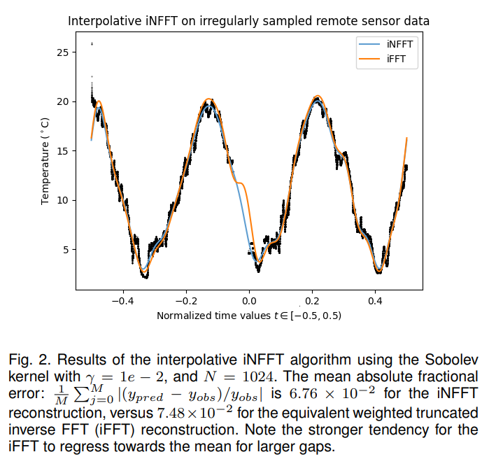
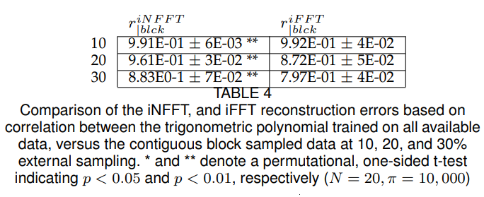
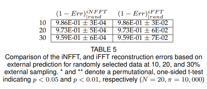
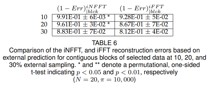
study for the iterative solution to the optimal interpolation problem. However, it is clear that a more critical metric for determining the accuracy of the interpolation is by removing contiguous blocks of data, and comparing the reconstruction against the true values for those data. Despite this, and considering that the interpolation was “smoothed” using a rather aggressive low-pass filter, the results are reasonable and corroborate that the calculated spectrum of the data is relatively consistent with what data is observed, which is consistent with what we would expect a true inverse transform to return.

The results also suggest that the interpolative algorithm performs significantly better relative to the equivalent truncated inverse Fast Fourier Transform (iFFT) using an equivalent number of coefficients and weight function in virtually all cases. The differences are most differentiated relative to correlation with the “true” underlying trigonometric polynomial, as shown in Tables 4 and Tables 4; only in the case of randomly sampled data is the difference inconsequential (Table 4). Despite poorer evidence of significance, on average the iNFFT algorithm in the most challenging use cases for up to 30% missing data.