

Authors:
(1) Michael Sorochan Armstrong, Computational Data Science (CoDaS) Lab in the Department of Signal Theory, Telematics, and Communications at the University of Granada;
(2) Jose Carlos P´erez-Gir´on, part of the Interuniversity Institute for Research on the Earth System in Andalucia through the University of Granada;
(3) Jos´e Camacho, Computational Data Science (CoDaS) Lab in the Department of Signal Theory, Telematics, and Communications at the University of Granada;
(4) Regino Zamora, part of the Interuniversity Institute for Research on the Earth System in Andalucia through the University of Granada.
Table of Links
Optimization of the Optical Interpolation
Appendix B: AAH ̸= MIN I in the Non-Equidistant Case
2 OPTIMIZATION OF THE OPTIMAL INTERPOLATION PROBLEM
2.1 With respect to the predicted Fourier coefficients, ˆf
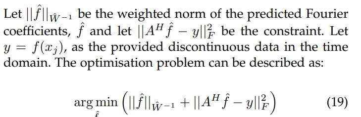
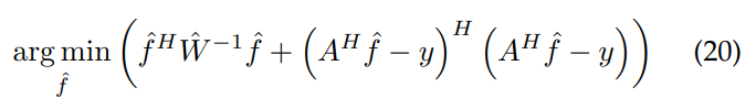
which through their respective norms is equivalent to:
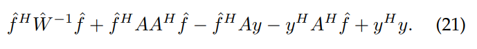
which unpacked as a polynomial expression:
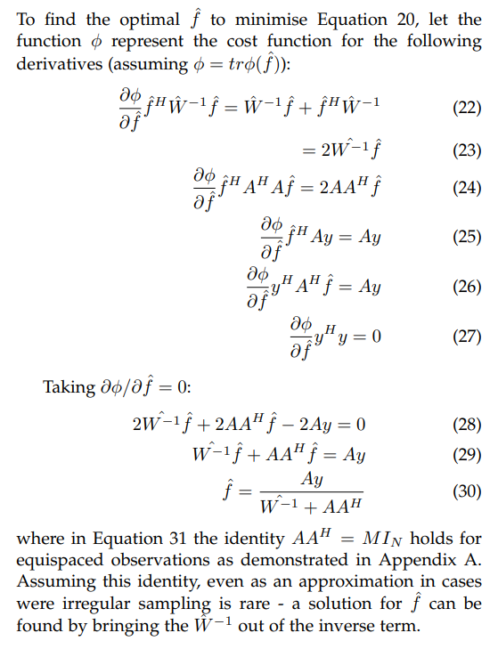
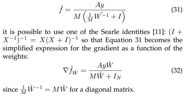
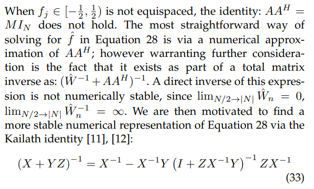
2.1.1 Optimal interpolation problem for equispaced nodes
Factoring out the constant M:
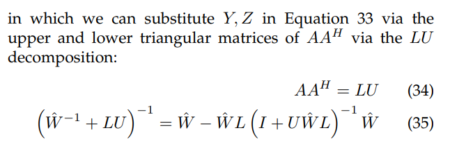
2.1.2 Optimal interpolation problem for non-equispaced nodes
substituting Equation 34 into the denominator of Equation 28, the function that minimises the cost function for the optimal interpolation problem as a function of ˆf in Equation 19:
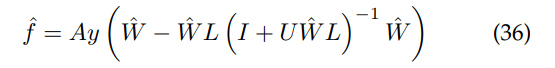
where it is clear that in Equation 36 we avoid the problem of directly inverting the kernel function along the diagonal of Wˆ , as a substitute for Equation 28.
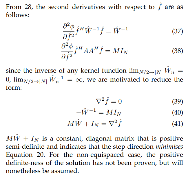
2.2 Second derivative test - equispaced case
This paper is available on arxiv under CC 4.0 license.