
Authors:
(1) Michael Sorochan Armstrong, Computational Data Science (CoDaS) Lab in the Department of Signal Theory, Telematics, and Communications at the University of Granada;
(2) Jose Carlos P´erez-Gir´on, part of the Interuniversity Institute for Research on the Earth System in Andalucia through the University of Granada;
(3) Jos´e Camacho, Computational Data Science (CoDaS) Lab in the Department of Signal Theory, Telematics, and Communications at the University of Granada;
(4) Regino Zamora, part of the Interuniversity Institute for Research on the Earth System in Andalucia through the University of Granada.
Table of Links
Optimization of the Optical Interpolation
Appendix B: AAH ̸= MIN I in the Non-Equidistant Case
Abstract
A simple least-squares optimization enables the determination of the spectrum for irregularly sampled data that is readily reconstructed using an adjoint transformation of the Non-Uniform Fast Fourier Transform (NFFT). This is an improvement upon previously reported iterative methods for such problems and is competitive in terms of time complexity with more recently proposed direct NFFT inversions when considering comparable matrix pre-computation steps. The software is highly portable, and available as a convenient Python package using standard libraries. Given its mathematical simplicity, however, it can be conveniently implemented on any platform.
Index Terms—Sensors, Digital processing, Non-uniformity correction, Remote monitor
1 INTRODUCTION
Remote sensor data is streamed from regions that are difficult to access for conventional measurements. Due to interruptions in either network connectivity, power or other environmental conditions there may be significant periods of time during which data acquisition is interrupted. This may not pose problems for ”binned” time-series analysis of the data, if the acquisition rate of the data is relatively high compared with the expected duration of a typical outage.
Binning data does partially resolve the spatio-temporal lag of phenomena measured across different points for the same event which is assumed to take place within a predefined period of time. However regardless of whether or not missing data is present, this does not make use of the full acquisition rate of the instrument, which negates some benefits of remote measurement. Instead, it is possible to perform an analysis of the spectrum or frequency domain information of the remote measurements and reconstruct the original data based on parallel analysis of similar remote stations.
Spectral analysis of irregularly sampled data is an active area of research, and is often referenced broadly as a leastsquares analysis, owing to a need for numerical estimation. This type of analysis commonly finds applications wherever there is an interruption in measurement - as is commonly seen in climate applications [1], and other environmental monitoring [2].
1.1 Fourier transforms of irregularly sampled data
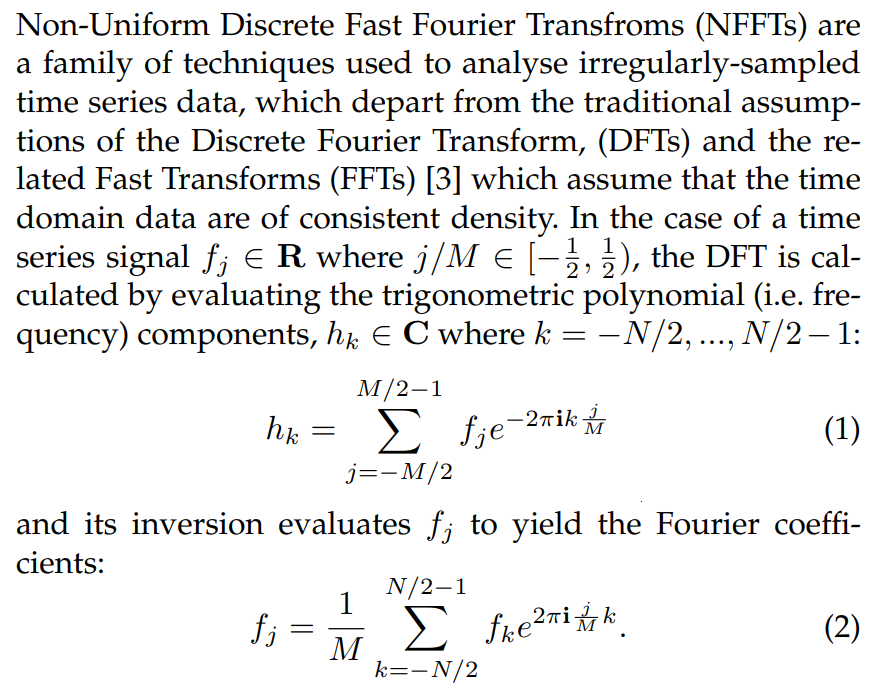
A full spectrum of Fourier coefficients in N can be calculated up to M = N where the maximum frequency of N/2 is the Nyquist frequency; beyond which the sampling rate is not sufficient to warrant calculation of further coefficients.
1.2 Non-Uniform Fast Fourier Transforms
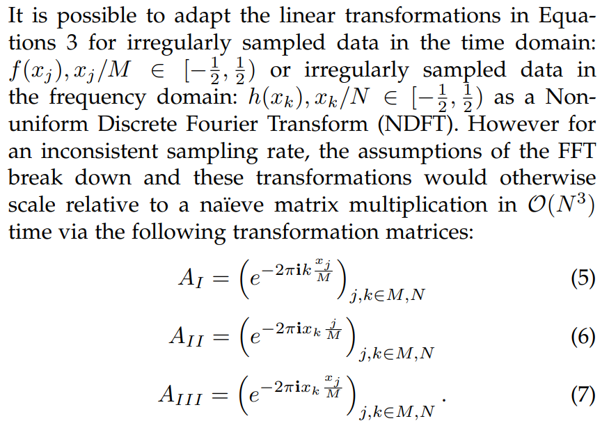
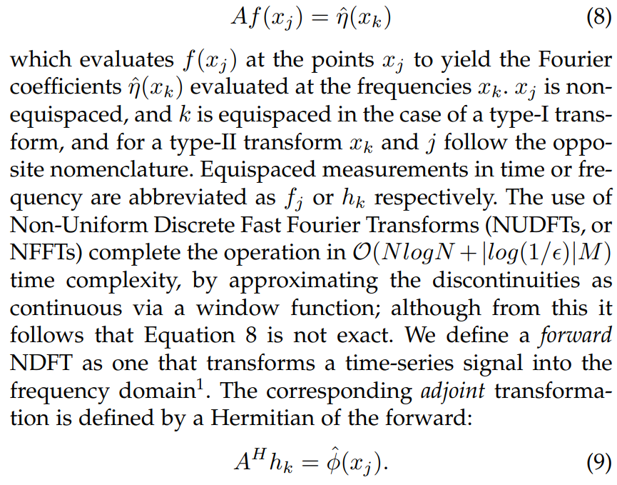
Equations 5, 6, and 7 refer to non-uniform transforms of types: I (irregularly-sampled time-series data; equispaced frequency-domain data), II (equispaced time-series data, discontinuous frequency-domain data), and III (discontinuous time and frequency-domain data) which are equivalent to the transform:
1.3 Inverse NFFTs
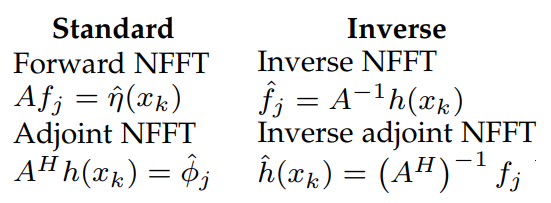
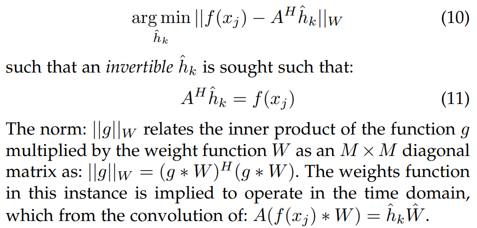
Inverting A directly via a pseudo-inverse is computationally inefficient, relative to the standard set by an inverse Fourier transform in the equidistant case. Rather, it is more convenient to find a series of Fourier coefficients such that the original time series data is recoverable via the adjoint transform. This can be done in the least squares sense by minimising:
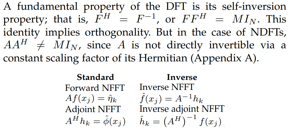
A number of proposals to solve this optimisation problem, and others have been put forward, but the method varies depending on the condition of the inverse problem, especially for direct solutions [9]. Tables 1.3 and 1.3 are provided to clear any potential confusion, for transformations of types I & II. For the purposes of this work and to explicate the far more common scenario where irregularly sampled time-series data are provided, the focus will be exclusively on type-I transforms, although it would be relatively straightforward to apply the same thinking to type-II transforms.
1.4 Optimal interpolation problem
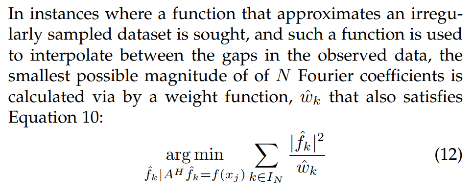
The optimal interpolation problem has been solved earlier using the Conjugate Gradient Method that minimises the successive error at each iteration, rather than the residuals relative to the original data [10].
This work demonstrates the quadratic form of Equation 12, and offers a convenient method for solving the interpolative iNFFT without the need to iterate. In addition, it avoids problems with dimensionality by inverting the AAH matrix, which sacrifices time complexity for simplicity; this is an acceptable trade-off for small values of N and competitive with faster algorithms for the direct inversion of non-uniform fast Fourier transforms which require similar O(N2 ) matrix pre-computations [9].
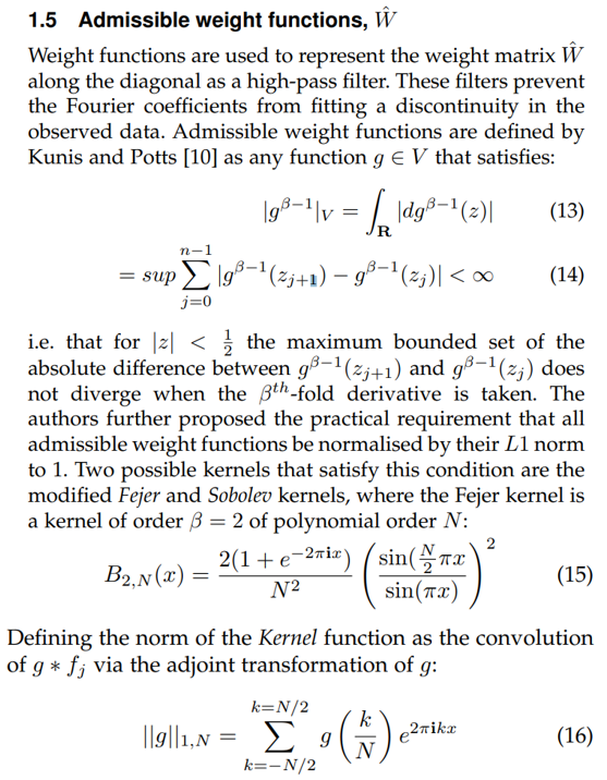
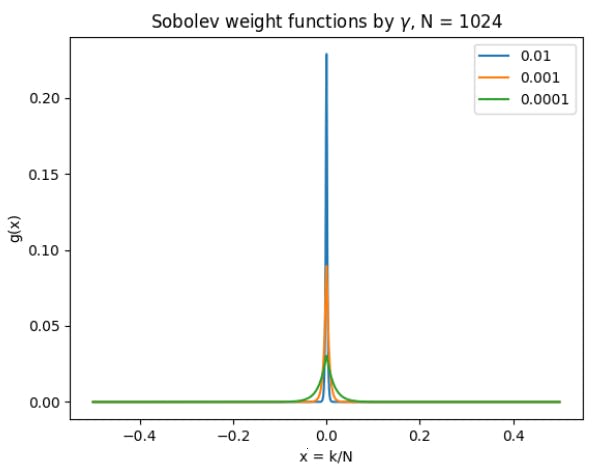
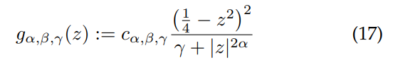
can be used to define the Sobolev kernel, first as an intermediate and generalisable weight function:
This paper is available on arxiv under CC 4.0 license.